SUM Excel Strategies for BIM Data Analysis

As we're getting ready to release our upcoming training program (The BRIDGE) on Quantity and Cost Analysis from Archicad to Excel, we wanted to prepare an intro training specific to SUM formulas.

The goal is to unpack the building blocks of some of the most useful SUM functions, so that you can build up formulas that SUM Quantity and Cost Totals to line items.

This is especially useful and important to understand, as once you do, it enables you to access large datasets with speed and precision, dialing in the summary data needed for extracting relevant quantities and cost information based on the criteria you select.

We've structured this tutorial into a 10 step process, building up the formulas as we go, from simple, to more advanced (and more powerful!).

Jump to the YouTube Video here.

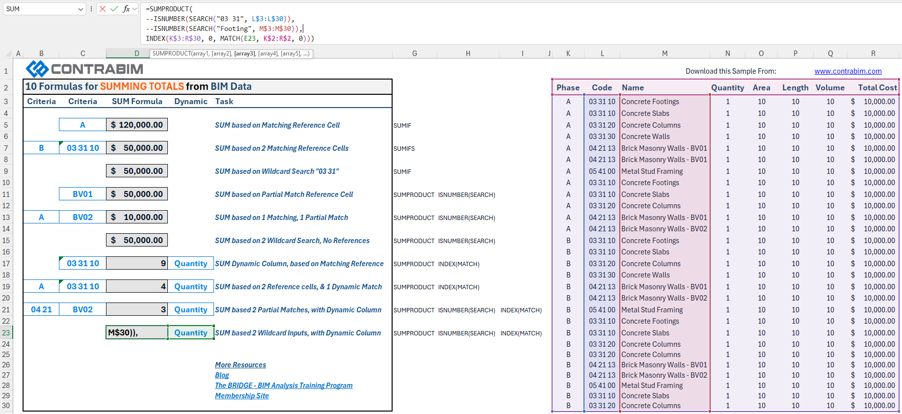
DOWNLOAD this sample Excel Form:

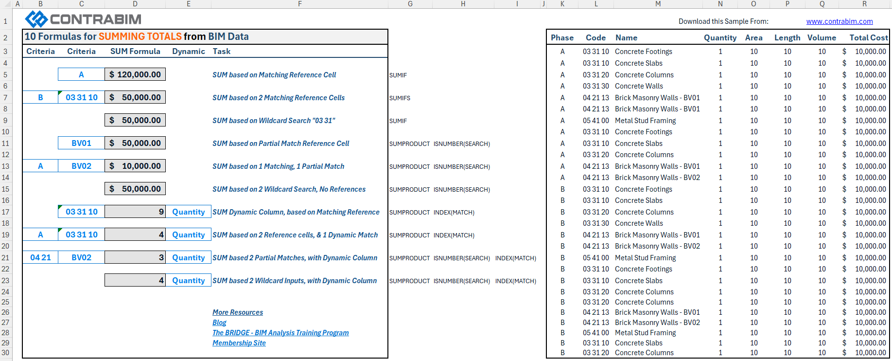
Key Functions used in Formulas:

SUMIF: Basic SUM function when 1 criteria is met, either direct cell reference (exact match), or wildcard search.

SUMIFS: Basic SUM functions with multiple criteria, of matching reference cells.

SUMPRODUCT: Expanded SUM function, enabling multiple arrays to be multiplied together, then summed into a total.

SEARCH: Function finds reference cell, or partial text within text.

ISNUMBER: Return TRUE when found

--      : Syntax used before ISNUMBER, to convert TRUE to 1, FALSE to 0

MATCH: Finds Dynamic Column

INDEX: Returns the correct Column

Criteria Types

Reference Cell Match: When a formula references the exact match from a cell

Reference Cell Partial Match: When a formula references a partial match (text found within text), from another cell.

Wildcard Search: Typed directly into a formula, with "*wildcard*" format in SUMIF formulas, or "wildcard" in SUMPRODUCT.

SUM Return Types

Static - Always pointing to the same column reference

Dynamic - Returns a column based on matching input (column header). By use of INDEX(MATCH)

Why this is important and relevant for BIM Data?

Building Information Models are constantly changing from conceptual design, to SD, DD, and Construction Documents. They evolve, and the data associated with elements evolves with it.

It's common for BIM data sets to expand in size, and contract, and will often be rearranged in order based on how the schedules are filtered and organized.

SUMIF/SUMPRODUCT formulas can be especially useful for extracting totals from the BIM Data sets, which may change and grow over time.

Having the ability to extract from a data table, based on specific criteria, the totals... is a powerful skill to master. 

Once you do, you then can tap into BIM data sets with ease and precision!

This is the whole point of "The BRIDGE" workflow we've developed at CONTRABIM, and the subject of our upcoming training series.

Consider the following tasks a SUMMING crash course!

HUGE IMPORTANT NOTE!!!

As we go through these tasks, we'll be using cell ranges, as noted by their columns and rows. This is useful for getting started, but it's not ideal for the long run.

The 2nd half of this article, will explore TABLES! Which are a powerful tool in Excel, and alternative method of entering formulas which make them much easier to manage, read and understand.

OK, let's get into it!

Task 1 (D5) - Return Summed Total based on 1 Matching Reference Cell (Exact Match)

If we only have 1 criteria to match, then a SUMIF is an easy and effective formula to use.

In this example, we'll use our Phase as our criteria range (Column K), "A" as an inputted criteria in cell (C5), and sum range as Total Cost (Column R)

=SUMIF(K$3:K$30, C5, R$3:R$30)

SUMIF(range, criteria, [sum range])

This formula will look in column K to find anymatching cell references in C5 (A), and return the summed total from column R (Total Cost).

Easy! 

Task 2 (D7) - Return Summed Total Based on 2 Matching Reference Cells (Exact Match) (D7)

SUMIFS, can handle 2 or more exact matching reference cells. This formula works the same way, but starts with the sum range.

=SUMIFS(R$3:R$30, K$3:K$30,  B7, L$3:L$30, C7)

SUMFS(sum_range, criteria_range1, criteria 1, [criteria_range2, criteria2], [criteria_range3, criteria3], etc...

Task 3 (D9) - SUM based on *Wildcard* Search (D9)

Instead of referencing a cell, in this case we'll manually type in the value we want to use as criteria.

This can be useful to extract a unique code, ID, term, manufacturer, product number... simple and effective.

=SUMIF(M$3:M$30, "*BV01*", R$3:R$30)

 We place *'s around the search term, then quotation marks around the stars when using SUMIF.

If you want to use SUMIF using a partial match, writing in the *Wildcard* search term into the formula is the best way to do this.

SUMIFS cannot reference a cell, and do a partial match. 

Which is where SUMPRODUCT comes in! 

Big Picture behind SUMPRODUCT

SUMPRODUCT enables us to have more complex criteria, including SEARCH terms, cell references, and formatted text extractions from cell references.

SUMPRODUCT works by multiplying arrays together from a single row, then adding all rows together.

When using this function to summarize totals into specific line items from BIM Data, we're often only looking for 1 column of data to be returned, and summed, such as a quantity or a cost total.

In other words, we only are wanting to SUM 1 array in most cases.

What's powerful about this, is we can use other multiple arrays within the SUMPRODUCT function, to act as criteria.

When the criteria is met, we want that array to equal 1.

1 * any  number, is that that same number.

ISNUMBER takes care of this for us, by return TRUE if criteria is met.

--ISNUMBER converts the TRUE, to a 1. FALSE to 0.

Multiple Criteria met = 

1 * 1 * Summing Column = Summing Column.

Only 1 Criteria met =

1 * 0 * Summing Column = 0

If any criteria is not met, then it's a 0 we're looking for. 0 * anything is 0, which works perfect for excluding rows from a SUMPRODUCT when our criteria isn't met.

By introducing criteria which returns a 1 or 0, we can easily extract meaningful totals with a few simple building blocks.

Task 4 (D11) - SUM Based on Partial Match Reference Cell

 OK, let's get into a SUMPRODUCT formula!

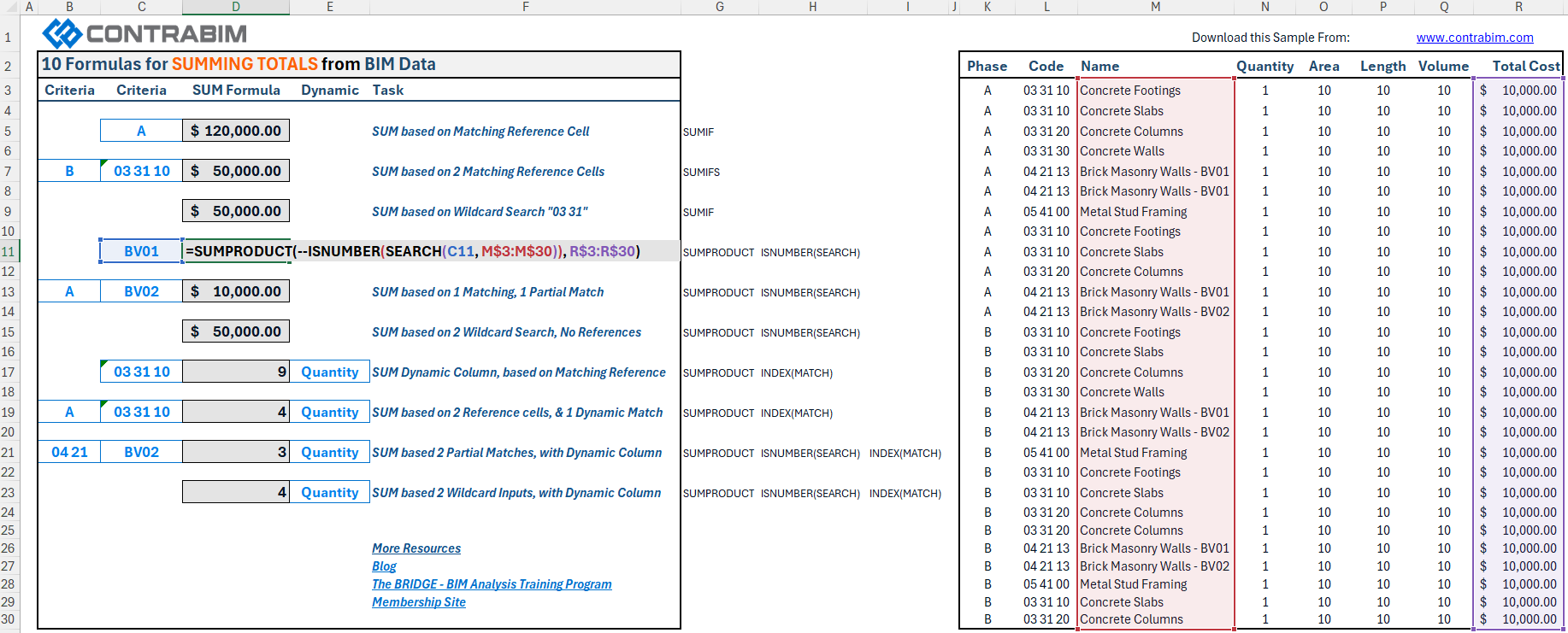
 =SUMPRODUCT(--ISNUMBER(SEARCH(C11, M$3:M$30)), R$3:R$30)

Array 1=      --ISNUMBER(SEARCH(C11, M$3:M$30))

Array 2=      R$3:R$30

Let's break down our array 1 formula (criteria).

C11 is our reference cell, which we're SEARCHING for within column M. If the search of the term found in C11 is found (BV01), then our criteria is met!

--ISNUMBER takes a matching criteria, and converts it to TRUE, and the (--) converts a TRUE to a 1.

Array 2 is the column we want to SUM in this case, the total cost.

Array 1 * Array 2 = Array 2

1 * $10,000 = $10,000

 This Array 1 is a powerful building block to our SUM workflow!

The order of arrays does not matter. These formulas return the same value.

=SUMPRODUCT(--ISNUMBER(SEARCH(C11, M$3:M$30)), R$3:R$30)

is the same as...

=SUMPRODUCT(R$3:R$30, --ISNUMBER(SEARCH(C12, M$3:M$30)))

Task 5 (D13) - SUM Based on 1 Reference Cell Match + 1 Partial Match

Let's look at another example, including a basic reference cell match, plus our partial match from the last task.

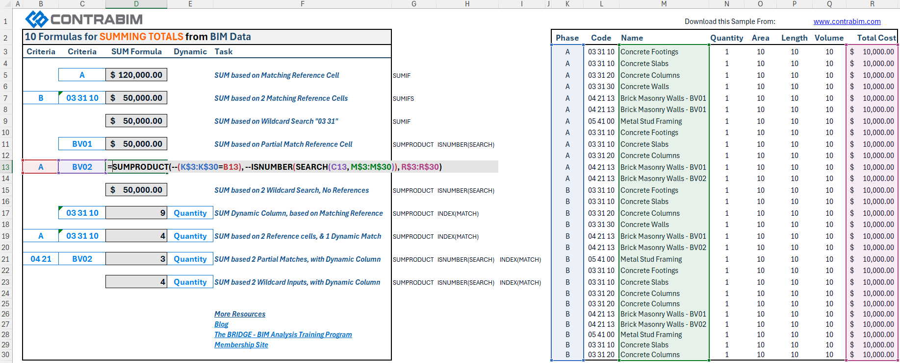
=SUMPRODUCT(--(K$3:K$30=B13), --ISNUMBER(SEARCH(C13, M$3:M$30)), R$3:R$30)

Array 1 = --(K$3:K$30=B13)

Array 2 = --ISNUMBER(SEARCH(C13, M$3:M$30))

Array 3 = R$3:R$30

Array 1, is searching with the range of K, for exact matching cell reference B13. Note, that the order doesn't matter across an equals sign.

K$3:K$30=B13        is the same as...     B13=K$3:K$30

These are being turned into a 1/0 with --( syntax.

Array 2 - Does this look familiar? It should, it's the exact same as our previous task.

Array 3 - Our target column for summing.

Task 6 (D15) - SUM Based on 2 Wildcard Searches

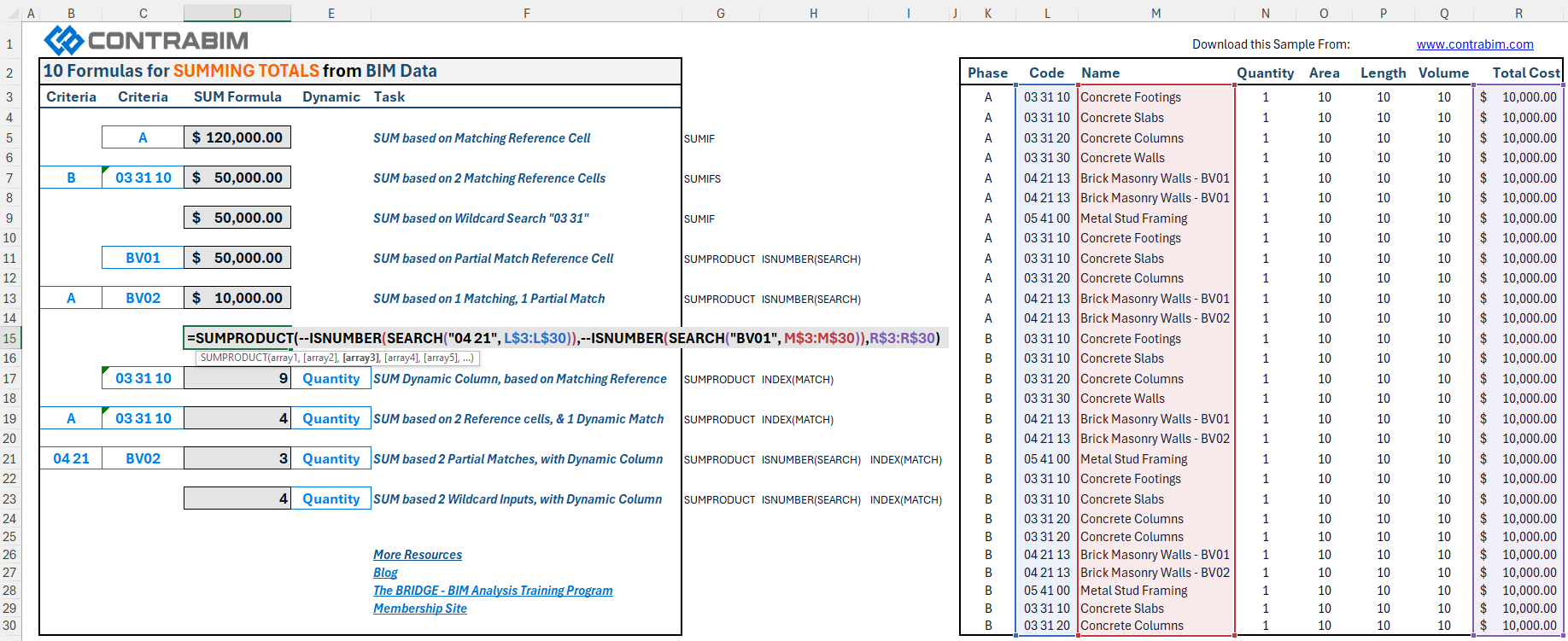
 =SUMPRODUCT(--ISNUMBER(SEARCH("04 21", L$3:L$30)),--ISNUMBER(SEARCH("BV01", M$3:M$30)),R$3:R$30) 

The formula above is 3 arrays, and it's starting to look more intimidating.

Using ALT-ENTER, we can add returns in our formula bar, making it easier to read.

=SUMPRODUCT(
--ISNUMBER(SEARCH("04 21", L$3:L$30)),
--ISNUMBER(SEARCH("BV01", M$3:M$30)),
R$3:R$30)

Each of the 3 arrays, is on it's own row below SUMPRODUCT(

Array 1 - Notice the Quotes around the Search Term "04 21". When not referencing a cell in this criteria, we need to use Quotes for a wildcard input!

Array 2 - Same as 1...

Array 3 - Sum Column

Hopefully these array building blocks are starting to make more sense!

Up until this point, we've been summing 1 specific column (Total Cost).

What if we want to introduce a variable? so that our column becomes more dynamic based on a certain reference cell input?

This is something we often come across, when there's different units of measurement being reported onto a row of a quantity takeoff schedule.

Sometimes we want counts (qty), sometimes areas (sf/m2), sometimes lengths (lf/m1), volumes, weights, heights, etc....

This is where introducing a Dynamic Column selection, based on a Unit, becomes extremely useful!

For this, we need to introduce our Index(Match) function.

INDEX (MATCH)

This combination of functions, enables us to find the matching column, based on an input.

Let's see how this works in the next task.

Task 7 (D17) - SUM w Dynamic Column, Based on Reference Cell Match

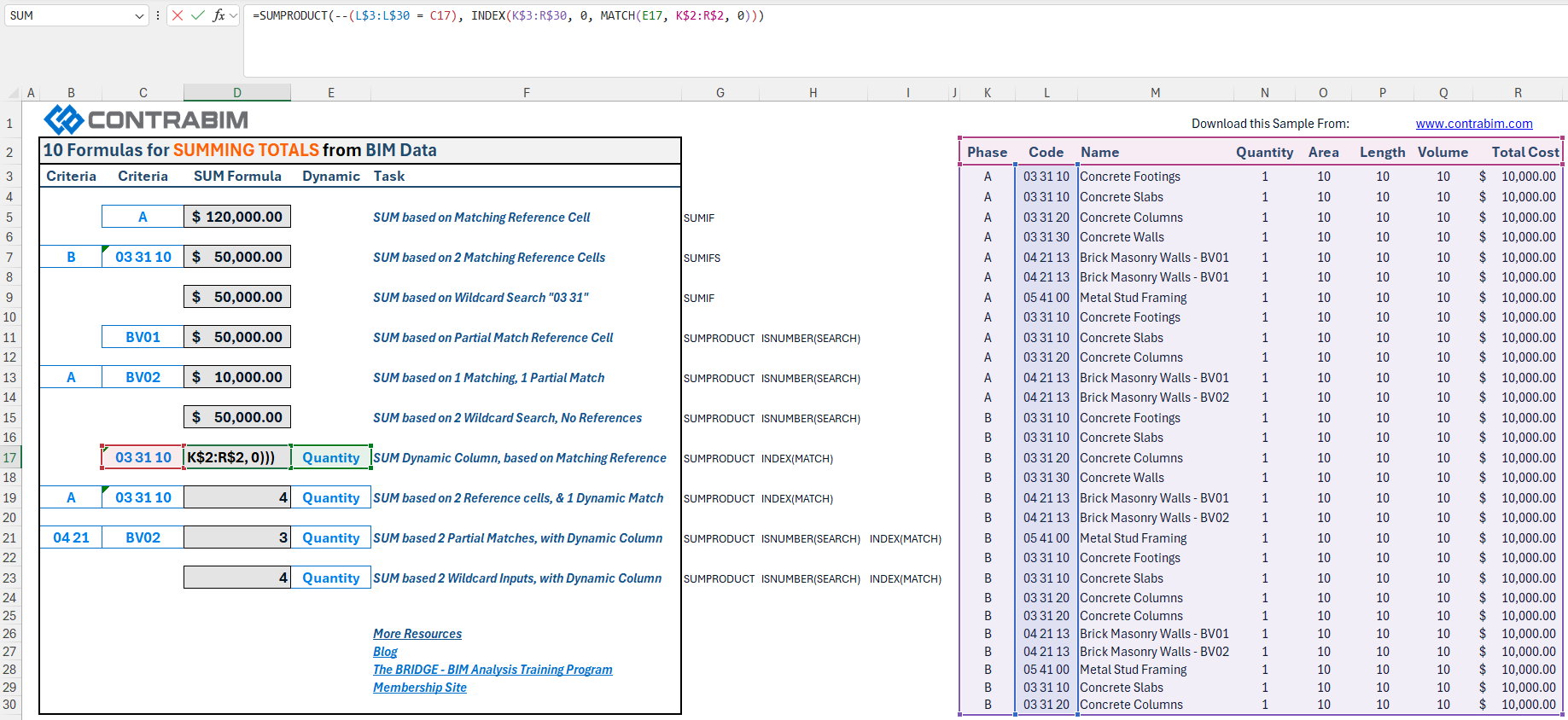
=SUMPRODUCT(--(L$3:L$30 = C17), INDEX(K$3:R$30, 0, MATCH(E17, K$2:R$2, 0)))

Array 1: --(L$3:L$30 = C17)

Array 2: INDEX(K$3:R$30, 0, MATCH(E17, K$2:R$2, 0))

Array 1, should look familiar. It's our criteria, being turned into a 1/0.

Array 2, references both our header, and entire data set.

 MATCH(E17, K$2:R$2, 0)

MATCH(lookup_value, lookup_array, match type)

The MATCH functions, finds our dynamic column, as indicated from cell E17. Match type is 0, for exact.

The INDEX references our entire table, without headers.

With this formula, we can choose which column gets returned based on our dynamic reference cell input, verse hard-coding into the formula!

This gives us the option to have 1 formula for a wide variety of columns, to be selected by a unit or type input reference cell.

Task 8 (D19) - SUM Dynamic Column, based on 2 Reference Cells

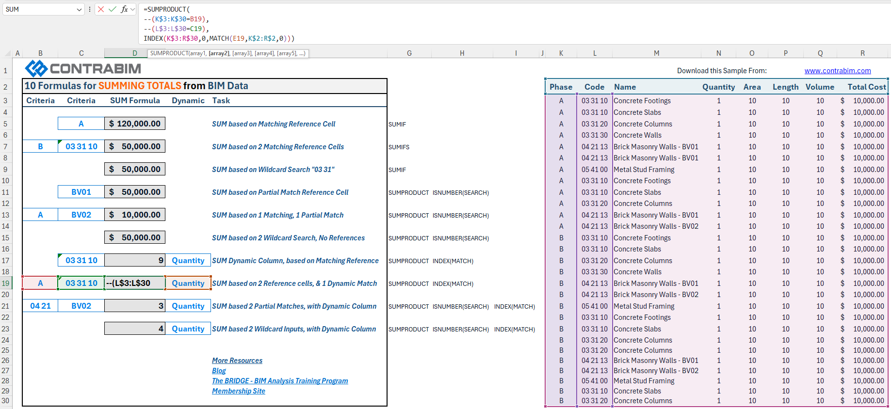
=SUMPRODUCT(
--(K$3:K$30=B19),
--(L$3:L$30=C19),
INDEX(K$3:R$30,0,MATCH(E19,K$2:R$2,0)))

Task 9 (D21) - SUM Dynamic Column, based on 2 Partial Matches

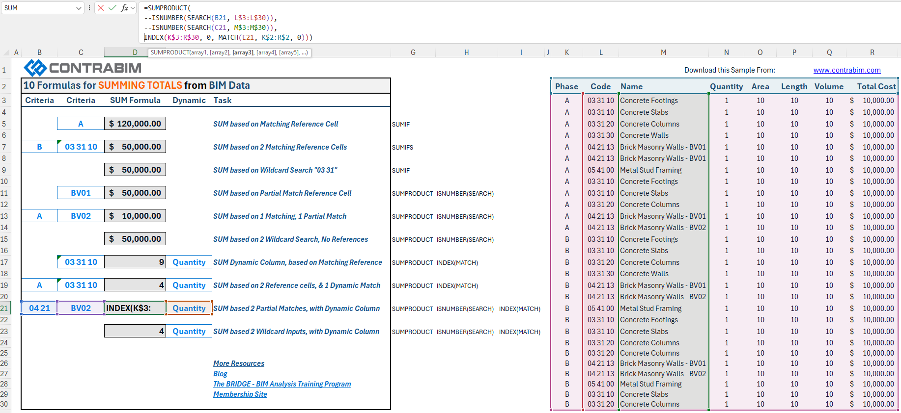
=SUMPRODUCT(
--ISNUMBER(SEARCH(B21, L$3:L$30)),
--ISNUMBER(SEARCH(C21, M$3:M$30)),
INDEX(K$3:R$30, 0, MATCH(E21, K$2:R$2, 0)))

Task 10 (D23) - SUM Dynamic Column, based on 2 Wildcard Searches

 =SUMPRODUCT(
--ISNUMBER(SEARCH("03 31", L$3:L$30)),
--ISNUMBER(SEARCH("Footing", M$3:M$30)),
INDEX(K$3:R$30, 0, MATCH(E23, K$2:R$2, 0)))

Creating TABLES in Excel

By selecting the entire dataset, including headers, we can easily convert our BIM Data from a range of cells, to a named table, using the "Insert Table" feature.

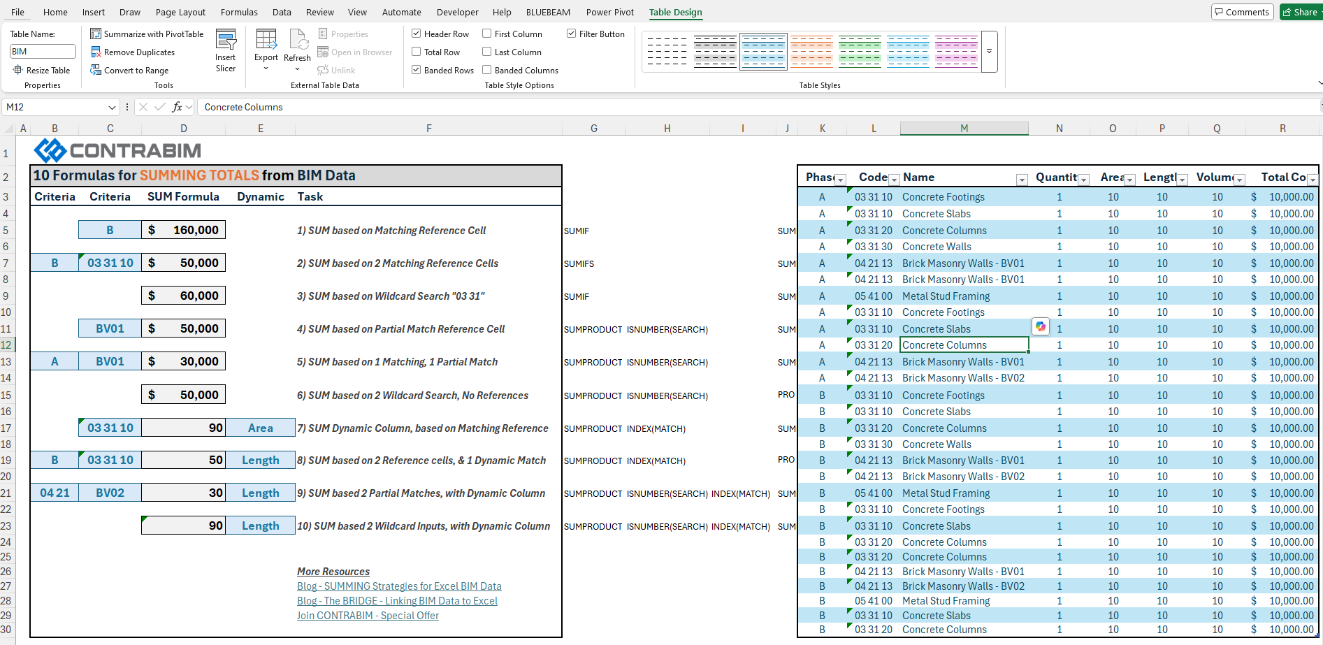
When clicking inside the table, you'll see the Table Design tab appear a the top of Excel. Here you can easily change the style, as well as resize the table if you need to make changes down the line.

When working with expanding data sets, it can be useful to oversize the table both in width and length, if you're updating your BIM data knowing your total rows and columns may increase in size.

Once a table is created, make sure to define the Table Name, in the top left corner of the Table Design tab.

This name will be important, as we can now reference the Table within our Formulas, INSTEAD of cell range!!!

When highlighting ranges within formulas directly to the Table, Excel will recognize that it is coming from a table, and replace the cell ranges with Table Name, and Columns.

So this formula (Task 1)

=SUMIF(K$3:K$30, C5, R$3:R$30)

Becomes...

=SUMIF(BIM[Phase], C5, BIM[Total Cost])

Much easier to read! No more guessing which column you're referencing.

Another sample (Task 10)

=SUMPRODUCT(
--ISNUMBER(SEARCH("Concrete",BIM[Name])),
--ISNUMBER(SEARCH("03 31 10",BIM[Code])),
INDEX(BIM, 0, MATCH(E23, BIM[#Headers], 0)))

Using a table, instead of cell ranges, makes it much easier to tap into the data set from across different sheets in your workbook.

Well that is it for this crash course on SUMMING BIM Data in Excel!

Want to learn more? Check out our upcoming training course "The BRIDGE".

Learn more about The BRIDGE

This course will show you how to setup Archicad for Quantity Takeoff, and also Excel for Quantity Analysis! From there, you can build any type of cost analysis outputs and summaries that you'd like.

The course is available for CONTRABIM Members, and will go live end of July/early August.

Not a member?

Join before August 1st, to save huge, as we mark our 3rd anniversary of our membership site.

JULY PROMO OFFER